In a previous post I talked to you about how you can use the power of linear algebra to solve big systems of linear equations (and even non-linear equations) and about how C++ linear algebra libraries such as Eigen can make your life easier by providing the data structures and algorithms for that purpose. But, wait a minute!!.. Why would someone want to solve big systems of equations? You probably remember inverting little systems of linear equations at school but the task was faster to carry out by using a pencil and a sheet of paper than by opening a computer and write a C++ program.
We’ll see today, with an interesting real life example, that inverting systems of linear equations is actually very useful because linear algebra problems are not just tables filled with numbers. They can also represent physical phenomena, or at least approximate the behavior of the “real world”. In many text books you’ll find the treatment of the heat equation as the basic example that perfectly illustrates that fact. In this post we’ll also start with the heat equation but add some extra “fun”: rather than simply study conductive heat flux in a given media, we’ll talk about the melting/solidification of a spherical ice/water ball.
The problem to be solved
Let consider a sphere of water. Suddenly this sphere is immersed in a cold atmosphere (say at any temperature lower than the melting temperature). In order to simplify the problem, we assume that the boundary of the sphere is suddenly at this cold atmosphere temperature. Also, no matter can be exchanged (there is no condensation/evaporation at the surface of the sphere). We finally suppose the sphere is small enough so that there is no convective displacement of water inside the drop/sphere. Conduction and phase change (solidification) are the only way heat can flow inside the domain.
For a given volume, we define the liquid fraction f as the proportion of this volume that is in the liquid state, the rest being solid.

Where ml is the mass of liquid in the volume of interest and ms le mass of solid.
We are interested in knowing the way the temperature and liquid fraction fields evolve with time in the sphere and we will use linear algebra to calculate it.
Problem formulation
One of my teachers in grad school often said that the trickiest part when dealing with a problem is to translate it into equations, then it is likely that someone already solved this kind of equation somewhere and you just have to apply (and understand) his method to find the solution to your own problem. This point of view is even more true when there are several possible mathematical formulations for a given problem: which one to pick? That’s what we’ll see here.
The north face
Most of you probably already heard about the heat equation, a partial differential equations that temperature field in a thermal media has to follow in order to comply with the laws of physics. The transient heat equation in a thermal media writes:

Where ρ is the material density, Cp is the heat capacity at constant pressure per unit of mass, κ is the thermal conductivity, t is time and T the temperature.
It looks like we identified the equation we were looking for, didn’t we? We just have to solve it in our sphere to get the temperature field and consider that the sphere is liquid when T>Tm (Tm being the fusion temperature, 273.15 K for water for example) and solid otherwise, right?
Well, it is not that simple. First of all, even if we assume that their thermal diffusivities are equal, solid and liquid water are a priori different thermal media and have different parameters values in real life. But that’s not the main concern, the really important issue is that the phase change is not thermally neutral and the latent heat of fusion/solidification needs to be captured somehow. Let Rm(t) be the position of the solid-liquid interface at t. The following formulation is then more accurate, assuming constant thermal parameters inside a given thermal media:

Where L in the latent heat of fusion per unit mass.
the first and second equations are respectively the heat equation in the solid and liquid phases whereas the third equation is the latent heat absorbed by the melting/solidification of ice.
This formulation is accurate but unfortunately it is not such an easy task to solve. The main reason being that tracking the interface between the liquid and solid phases is not trivial. So let’s look for an alternative
The enthalpy formulation
Let introduce the term of enthalpy which, in our case, can written as the sum of the “sensible” heat (i.e. linearly linked to the temperature, a variable one can “feel”) and the “latent” heat (that one cannot “feel”).
If we introduce it into the heat equation we get:

Where the enhtalpy h equals:

and this formulation is OK since it captures the latent heat!
Note that the enthalpy exhibits a discontinuity at the phase transition equal the latent heat of fusion per unit mass. As mentioned previously, most simulation methods really don’t like discontinuities. An easy and not that bad workaround consists in considering a smoothed version of the latent heat such as:

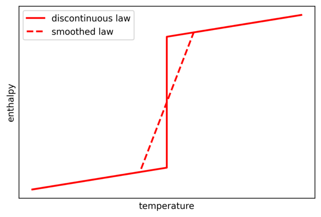
The domain is then divided into three states: solid, liquid and a “mushy” state in the smoothed area where liquid and solid phases coexist.
It seems that we have our problem put into equations, congratulations we’ve done the trickiest part! Let’s try to see if particularities of our problem allow us to simplify the formulation.
Remember that we are looking at the evolution of temperature and phases of a spherical ice/water particle subject to a uniform constant temperature over its surface. So we can study the problem in a spherical coordinate system centered in the center of the sphere.
Knowing that the physical parameters such as the thermal conductivity and the heat capacity are assumed to be constant and uniform, and that the particle is initially homogeneous, one can observe that the problem is invariant in rotation around any axis that passes through the sphere’s center. We can thus rewrite the equation (in a spherical coordinates system):


Finally, physicists adore physical parameters that have dimensions and units but mathematicians and computer scientists prefer to work with non-dimensional equations. Let consider the following variable changes that will make our lives so much easier:


Let also consider the Stefan number, a dimensionless parameter that is useful for studying phase change problems:

Te being the external temperature that is assumed to be instantaneously imposed at the boundary of the sphere at t=0.
Then comes:

Where:

And with the following initial and boundary conditions:


We have a well posed problem.
Numerical approximation
The good news is that we have a mathematical formulation of the problem to solve, the bad news is that it does not have a priori an easy analytical solution (actually it’s a good thing, otherwise we would not need linear algebra!). That’s where we thank the brilliant mathematicians who found a way (actually several ways) to get an approximation of the solution on a discretized subsets of the spatial domain and of the time interval: the finite difference methods (a.k.a FDM). In particular we will study the Crank-Nicolson method.
The principle is the following:
- descretize the spatial domain and time interval, that is, instead of considering [0,1] x [0,τend] consider {z0, z1, …, zn} x {τ0, τ1,… , τm}
- approximate derivatives with differences, that is:


Instead of finding the continuous temperature field θ(τ,z), we will find a vector for each τk. In the previous sentence, there is a word that certainly sounds familiar to you if you know linear algebra: the word “vector”.
It looks like we are getting closer! Let’s write now our equation at a given location for a given time step:

let’s act recursively and consider that you already know the temperature at the previous time step n and let then move all the unknowns on the left hand side and the known temperature values on the right hand side:

Don’t you see it coming? Yes, it looks like matrix algebra! For those who do not see, let re-write the same equation again:

Where f is a linear application (another matrix) and:


Wonderful, we have a linear system of equations!
Acutally I cheated a little bit because the thermal conductivity depends on the temperature (in the “mushy” zone it depends a lot on the temperature but not so much elsewhere), it is then non-linear (though quasi-linear almost everywhere), We add then another layer of approximation by linearizing the problem by using the old value for kappa (based on θi,n instead of θi,n+1). most of the time it is not a major approximation so it’ll be fine.
We only need to close the system by providing boundary conditions (the first and last rows of the matrix) and we are all set:


Numerical implementation
The following C++ lines provide an implementation of the resolution of the algebraic equations
We use a class that will carry all the logic. This class has few attributes, each representing a key parameter of the problem (e.g. number of spatial and temporal steps, Stefan number, etc. See the commented code below) and members that break down the work into elementary steps:
#include <fstream>

template <typename Vect, typename ParMat, typename ParVect>
class melt_sphere {
private:
    int M; // number of space steps (-)
    int N; // number of time steps (-)
    double dx; // non-dimensional space step (-)
    double dt; // non-dimensional time step (-)
    double dtheta; // non-dimensional semi-interval for mushy ice (-)
    double end_time; // end of simulation
    double Te; // non-dimensional external temperature (-)
    double stefan_number; // Stefan number (-)
    ParVect param_beta; // array of normalized parameter beta (-)
    Vect a,b,c,f; // three-diagonal and right-end vectors
    // private methods
    void generate_sparse_matrix(int ts);
    void generate_right_hand(int ts);
    void generate_beta(int ts);
    double beta(double theta); // help function for generate_beta
    void lu_factorization();
    void backward();
    void forward();

public:
    melt_sphere(int m, int n,
                     double et, double deltaT, double stef);
    ParMat sol; // matrix that store the temperature solution
    // note that this is for illustration purpose only because
    // it necessitates a lot of memory! DO NOT do such things in
    // production
    void save_in_file(std::string file_name);
    void solve();
};
Note the re-use of the lu_factorization, backward and forward functions from a previous post. Note also the use of template classes in order to be able to use any kind of Matrix and vector class (C++ std::vector or Eigen or the one of your choice).
The lines bellow show the implemntation of the methods of the melt_sphers class. First, the constructor:
template <typename Vect, typename ParMat, typename ParVect>
melt_sphere<Vect,ParMat,ParVect>::melt_sphere(int m, int n,
                     double et, double deltaT, double stef){
M = m;
N = n;
dx = 1./m;
end_time = et;
dt = end_time/n;
dtheta = deltaT;
Te = 0.;
ParMat solTemp(n+1, Vect(m+1));
sol = solTemp;
// HACK: here we add a 1.01 to dtheta in order to make sure the
// initial state is solid and not mushy
std::fill(sol[0].begin(), sol[0].end(), 1.+dtheta*1.01);
Vect aTemp(M,1.);
a=aTemp;
Vect bTemp(M+1,1.);
b=bTemp;
Vect cTemp(M,1.);
c=cTemp;
Vect fTemp(M+1,0.);
f=fTemp;
param_beta.resize(M+1);
stefan_number = stef;
}
The next method save the result in a txt file:
template <typename Vect, typename ParMat, typename ParVect>
void melt_sphere<Vect,ParMat,ParVect>::save_in_file(std::string file_name){
  std::ofstream temp_file(file_name + "_temp.txt", std::ios::out | std::ios::trunc);
  if(temp_file)
  {
      for(int i=0; i<M+1; i++){
          for(int j=0; j<N+1; j++){
              temp_file << " " << sol[j][i];
          }
          temp_file << std::endl;
      }
    temp_file.close();
    }
  else
  {
    std::cerr << "Error while opening the text file." << std::endl;
  }
}
then the algebraic problem to solve is put in place:
template <typename Vect, typename ParMat, typename ParVect>
void melt_sphere<Vect,ParMat,ParVect>::generate_sparse_matrix(int ts){
ParVect r = param_beta*dt/(2.*dx*dx);
b[0] = 1.0;
c[0] = -1.0;
for(int i=1; i<M; i++){
    a[i-1] = -r[i]*(1.-1./i);
    b[i] = 1.+2.*r[i];
    c[i] = -r[i]*(1.+1./i);
}
a[M-1]=0.;
b[M] =1.;
return;
}

template <typename Vect, typename ParMat, typename ParVect>
void melt_sphere<Vect,ParMat,ParVect>::generate_right_hand(int ts){
ParVect r = param_beta*dt/(2.*dx*dx);
f[0]=0.0;
f[1]=(1.-2.*r[1])*sol[ts][1]+r[1]*(1.+1./1.)*sol[ts][2];
for(int i=2; i<M; i++){
    f[i]=r[i]*(1.-1./i)*sol[ts][i-1]+(1.-2.*r[i])*sol[ts][i]+r[i]*(1.+1./i)*sol[ts][i+1];
}
f[M] = Te;
return;
}

template <typename Vect, typename ParMat, typename ParVect>
double melt_sphere<Vect,ParMat,ParVect>::beta(double theta){
double res;
if(theta > 1.+dtheta){
    res = 1.;
}
else if(theta < 1.-dtheta){
    res = 1.;
}
else{
    res = 1./(1.+stefan_number/(2.*dtheta));
}
return res;
}

template <typename Vect, typename ParMat, typename ParVect>
void melt_sphere<Vect,ParMat,ParVect>::generate_beta(int ts){
for(int i=0; i<M; i++){
    param_beta[i] = melt_sphere<Vect,ParMat,ParVect>::beta(sol[ts][i]);
}
return;
}
and fnally solved after LU factorization:
template <typename Vect, typename ParMat, typename ParVect>
void melt_sphere<Vect,ParMat,ParVect>::lu_factorization(){
c[0]=c[0]/b[0];
b[0]=b[0];
for(int i=1; i<M; i++){
    b[i]=b[i]-a[i-1]*c[i-1];
    c[i]=c[i]/b[i];
}
b[M]=b[M]-a[M-1]*c[M-1];
}

template <typename Vect, typename ParMat, typename ParVect>
void melt_sphere<Vect,ParMat,ParVect>::forward(){
f[0]=f[0]/b[0];
for(int i=1; i<M+1; i++){
    f[i]=(f[i]-a[i-1]*f[i-1])/b[i];
}
}

template <typename Vect, typename ParMat, typename ParVect>
void melt_sphere<Vect,ParMat,ParVect>::backward(){
for(int i=M-1; i>=0; i--){
    f[i]=f[i]-c[i]*f[i+1];
}
}

template <typename Vect, typename ParMat, typename ParVect>
void melt_sphere<Vect,ParMat,ParVect>::solve(){
for(int i=1; i<=N; i++){
    melt_sphere<Vect,ParMat,ParVect>::generate_beta(i-1);
    melt_sphere<Vect,ParMat,ParVect>::generate_right_hand(i-1);
    melt_sphere<Vect,ParMat,ParVect>::generate_sparse_matrix(i-1);
    melt_sphere<Vect,ParMat,ParVect>::lu_factorization();
    melt_sphere<Vect,ParMat,ParVect>::forward();
    melt_sphere<Vect,ParMat,ParVect>::backward();
    sol[i]=f;
}
}
Here is an example of a main function that would instantiate the melt_sphere class in order to solve a sphere solidification problem using either default parameter or user defined arguments. The std::vector and std::valarray data structures are used:
#include <vector>
#include <valarray>
#include "sphere_phase_change.cpp"

typedef std::vector<double> Vect;
typedef std::vector<std::vector<double>> ParMat;
typedef std::valarray<double> ParVect;

int main(int argc, char* argv[]){
int M, N;
double stef, k, et;

if(argc==6){
    M = std::stoi(argv[1]); // number of length steps (-)
    N = std::stoi(argv[2]); // number of time steps (-)
    // environmental conditions
    stef = std::stod(argv[3]);
    k = std::stod(argv[4]); // dtheta (-)
    et=std::stod(argv[5]); // end time (-)
}
else{
    M=400; // number of space steps (-)
    // environmental conditions
    stef = 1.;
    k = 0.1; // dtheta (-)
    // time information
    et=0.3; // end time (-)
    N=400; // number of time steps (-)
}

double end_time=et*stef; // end time (-)
double dTemp=k; // non-dimensional dtheta [-]

std::string file_name="solidification";


melt_sphere<Vect,ParMat,ParVect> prob(M, N, end_time, dTemp, stef);
prob.solve();
prob.save_in_file(file_name);

return 0;
}
Comparison with the litterature
I got this example from a paper by Caldwell and Chan where they studied the solidification of a sphere of water and compared the enthalpy method’s performances Vs another method. The benchmark between the two methods is assessed via the phase change front position as a function of time for three different Stefan number values. They conclude that the enthalpy method compares well with Heat Balance Integral Method (which is their reference and that we will not detail here) even though it has a tendency to lower it’s accuracy for some values of the Stefan number. Let’s compare our results with Caldwell and Chan’s.
Before doing that, note that the way I implemented the resolution is much more basic and simple than the one used by Caldwell and Chan. Actually I was inspired by another paper by deWitt and Baliga issued by Nasa back in the 80s. Just so you know, here too I added a layer of simplification in the application of the Crank-Nicolson method, besides in deWitt and Baliga’s paper they do not treat a spherical domain so I also had to adapt the equations.
If you looked carefully at the way I simplified the problem and linearized the enthalpy discontinuity you probably noticed a potential degree of freedom in my formulation: Δθ. Engineers love adjusting their models using such degrees of liberty, a.k.a. “knobs”, but scientists don’t because that’s how you sweep the dust under the rug. In “real life” the h=f(T) function is discontinuous and the linearization I put in place is a numerical artefact. So as Δθ tends to 0, h gets closer to its actual form but you cannot get an accurate numerical solution whereas when Δθ gets bigger your numerical resolution is easier but you get further to reality.
Here we study different values for Δθ and compare the best compromise we find with the references from Caldwell and Chan (in red). In blue is the "mushy zone" I calculate. There water is neither liquid nor solid and that's where the phase change happens:
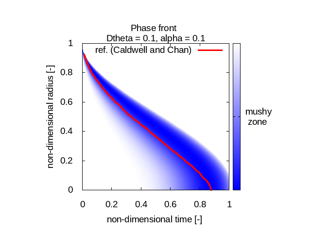
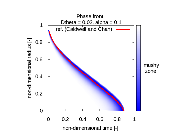
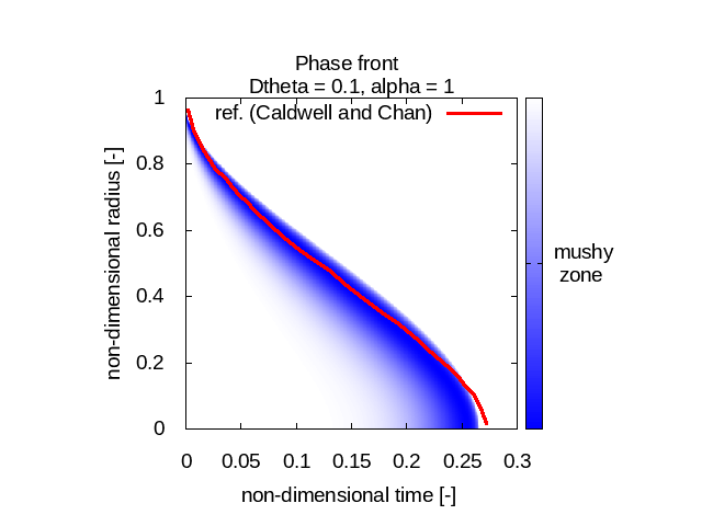
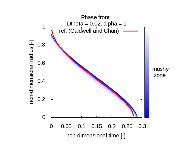
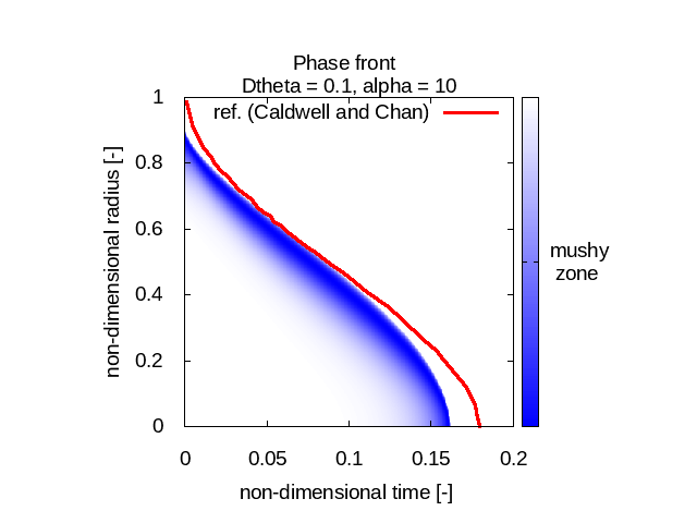
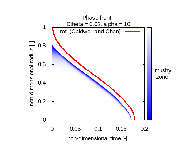
The first observation is that our model behaves differently for different Stefan number values. For relatively small Stefan numbers (0.1 and 1) our model fits quite well with Caldwell and Chan’s reference phase front curves (no matter Δθ) whereas when the Stefan number is relatively high (10) the results we get don’t match at all the expected physical behavior.
The other observation we can do is that the implementation I used seems to diffuse the “mushy zone”, that is this fictitious uncertainty area where the phase is somewhere between liquid and solid.
If you are interested, you can find all the code of this post on my github, feel free to re-use and improve it.
Also the references I cited in this post are both freely available online:
- Caldwell, J., & Chan, C. C. (2000). Spherical solidification by the enthalpy method and the heat balance integral method. Applied Mathematical Modelling, 24(1), 45-53
- DeWitt, K. J., & Baliga, G. (1982). Numerical simulation of one-dimensional heat transfer in composite bodies with phase change (No. NAS 1.26: 165607)
Have fun!