Eigen is a C++ linear algebra library that is especially designed to help you efficiently perform heavy algebric operations such as matrix and vector calculations. It is particularly useful when you need to solve a (big) system of equations: that is typically what you want to do when you solve a discrete approximation of a differential equation. I will touch base on this specific application of linear algebra in a future post. For now, let’s focus on what is linear algebra from a general perspective, why it is a powerful tool and how Eigen can make your life easier.
Let’s talk about what is linear algebra first
When dealing with the numerical resolution of a system of equations, if your problem is relatively small, you may decide to implement your own data structure and algorithm (for example the substitution method, widely taught at school) and it will probably be fine at the beginning. But as the number of unknowns grows, you’ll soon be overwhelmed by the cognitive limits which will prevent you from managing each unknown individually, not even talking about memory or performance issues (and most likely by both). That’s when linear algebra comes along, a sort of one-size-fits-all abstraction, a framework that free you from micro-managing each individual equation of your system. You just need to master the big picture, make sure it respects a set of properties and that’s it! Take the following system of equations for example:

Using linear algebra it becomes:

That can be written:

Much easier to apprehend, isn’t it? More importantly, all linear systems can be written that way, all you need to do is changing the sizes and the values of the table A (called a matrix) and the array b (called a vector, like the array of unknowns x). formally, every linear system of equations is strictly equivalent to a linear mapping between two vector spaces. Once again, that’s awesome because it means that we do not have to reason at the «microscopic scale» anymore. Nowadays it is really common to solve systems of equations with billions of unknowns.
That being said, I only told you that your linear system of equations can be written in a simpler way… but I did not tell you how to solve it. That’s when it becomes interesting, provided your linear mapping, or equivalently your matrix, has a certain set of properties (easy to assess most of the time), you will be able to determine if your system of equations has 0, 1 or several solutions. Finally, a bunch of mathematical techniques exist (that range from super easy to super difficult to implement numerically) that you can apply in order to get a solution to your problem.
Bonus: even if linear algebra, by definition, deals with solving linear problems (i.e. made of additions of unknowns multiplied by constant coefficients) many brilliant mathematicians found various methods to approximate the resolution of non-linear problems by the resolution of successive linear problems, much easier to solve thanks to guess what… linear algebra!
let’s come back to your problem
Now you know that there are powerful mathematical tools to solve it. You could roll your sleeves up and use the built-in C++ array as a base for your own vector and matrix classes and implement yourself various resolution techniques… that’s indeed doable and many people do that. Besides it’s a good exercise if you want to learn and understand in details those methods. However, odds are that once again you’ll reach some memory and/or performance limitations as the number of unknowns grows. It is likely that your implementation will not optimal, especially if you are a beginner or intermediate C++ developer.
Moreover, remember this old software engineering adage: «don’t reinvent the wheel». Starting from scratch takes a lot of work from designing to coding and testing… and often brings little value. Unless you are a linear algebra library designer (which is probably not the case, otherwise you would not be reading those lines), inverting linear systems of equation is not a goal as such, but rather a (potentially painful) step in «your» value creation process.
That’s when Eigen enters the room.
Eigen is an open source C++ linear algebra library that offers easy-to-use interfaces to create and manipulate matrices and vectors, it also comes with a full catalog of powerful algebraic problems resolution and decomposition routines.
Before we illustrate the power of Eigen with an example, let’s say a word or two about its installation procedure: super easy! (told ya: two words!). Indeed, you’ve basically almost nothing to do: Eigen is a pure header library, which means there are only .h files and no separate .cpp files. So all you need to do is to download and save the desired version of Eigen where you want in your system and locate the Eigen sub-directory inside the newly downloaded directory. This sub-directory contains all the aforementioned header files. Then you only have to #include the desired .h file at the beginning of your own C++ files. On my Linux system for example, I saved it in the /usr/local/include directory but I could have saved it in any directory listed in my LD_LIBRARY_PATH (that is a list of places systematicaly scanned by the compiler when looking for libraries).
We will now compare the performances of Eigen at solving a linear system of equations Vs a "handcrafted" solving implementation. Let’s go back to the previous example. I told you previously that there are plenty of techniques to solve linear problems. One of them is the LU decomposition. The principle of LU decomposition is that you decompose your problem into two interlinked "triangular" problems. Triangular problems are straight forward to solve because they can be treated as a succession of linear 1D 1 unknown problem. In linear algebra terms, LU decompostion is a factoryzation of M into a product of two triangular matrices: one lower triangular matrix (L), one upper triangular matrix (U).

As I said, LU decomposition is far from being the only available technique that could help you solving linear systems of equations. Like any method it has pros and cons. To be honest I picked this mostly because it is very widely used and also because I knew how to program it myself… let assume you are in a sitatuion where, for some reasons, LU decomposition is not satisfaying, what would you do? You would look for an alternative, identify the most relevant methods and implement them yourself in order to assess which one better meets your needs?.. Again it would mean a significant effort (do not forget that once you converged to something self implemented, you need to think about testing etc… good luck). Whereas a linear algebra library such as Eigen, offers a wide catalog of solvers and decompositions that you can try out very easyly (almost plug-n-play) and of which you can trust the robustness.
An handcrafted implementation of LU decomposition
Let start with the handcrafted implementation of the LU decomposition and resolution of a random system of M equations of M unknowns. The global approach is given by the folowing main function.
#include <iostream>
#include <chrono>


int main(){
srand(time(NULL));
const int M=640;
std::cout << "Matrix size M: " << M << std::endl;
auto tbegin = std::chrono::high_resolution_clock::now();
double L[M][M], U[M][M], b[M];

fill_dense(L, U, b);

lu_factorization(L, U);
forward(L, b);
backward(U, b);

auto tend = std::chrono::high_resolution_clock::now();
std::chrono::duration<float> duration = tend-tbegin;
std::cout << "execution time (s): " << duration.count() << std::endl;
return 0;
}
First things come first, as we want to compare the time performance of different methods, we define tbegin as the starting time of our chronometer. Then, we need to declare and fill the Matrices and vectors we will manipulate. M is the size of the system and we declare L, U and b that are respectively two matrices and a vector of size MxM (resp. M). The naming is transparent and you recognise the two matrices resulting from the LU factorization and the right-hand side of the algebraic equation to solve. That’s all the memory we will use. I already imagine your question «Wait! Where is the left-hand side (M.x) of the algebraic equation we are solving?» Actually when you deal with large size systems memory is expensive and you want to minimize its usage so as we do not use all these variables at the same time, we will recycle and use the memory allocated to U and b several times: we can then use aliases for educative purpose but it is not mandatory. Globally the space complexity of this code is O(N^2).
The next step is to fill the memory we just allocated, with the fill_dense funciton.
template <size_t N>
void fill_dense(double (&rL)[N][N], double (&rU)[N][N], double (&rb)[N]){
srand(time(NULL));
for (size_t i=0; i<N; i++){
    for (size_t j=0; j<N; j++){
        rU[i][j]= rand() % 9 + 1;
        rL[i][j]= 0.;
    }
    rL[i][i]= 1;
    rb[i]=1;
}
}
L is initialized with the identity matrix, that’s straight forward. Regarding A (a.k.a. U) and b we simply randomly fill them with an integer between 0 and 9. I know that nothing guarantees that this randomly generated matrix respects the conditions for being LU factorizable, let assume that when N is sufficiently high (say higher than 10) it is likely that all the conditions are united). Little note about srand(time(NULL)): it seeds the pseudo random number generator that the rand function uses. The time complexity of the fill_dense function is O(N2).
Now, the LU factorization per say starts with the LU_factorization function.
template <size_t N>
void lu_factorization(double (&rL)[N][N], double (&rU)[N][N]){
for (size_t n = 0; n < N; n++){
    for (size_t i = n+1; i < N; i++){
        rL[i][n]=rU[i][n]/rU[n][n];
    }
    for (size_t j = n+1; j < N; j++){
        for (size_t k = 0; k < N; k++){
            rU[j][k]=rU[j][k]-rU[n][k]*rL[j][n];
        }
    }
}
}
Say good bye to the A matrix because its content will be overiden by the U upper triangular matrix. Here we follow the Gaussian elimination technique to obtain the L and U matrices. This function, even though it is short, is the meat of the code. The time complexity of this part is O(N^3).
Remember that now, our system of equations can be written as in the following equation:

Where y = Ux is an intermediary variable for which, as you probably guessed, we will not use additional memory and simply recycle the b vector (a.k.a. x). To get the global solution x of the problem we simply have to solve two nested triangular systems of equation by forward-backward substitution. The cumulated time complexity of the two following functions is O(n^2).
template <size_t N>
void forward(double (&rL)[N][N], double (&rb)[N]){
for(size_t i=1; i<N; i++){
    for(size_t j=0; j<i; j++){
        rb[i]=rb[i]-rb[j]*rL[i][j];
    }
}
}

template <size_t N>
void backward(double (&rU)[N][N], double (&rb)[N]){
rb[N-1]=rb[N-1]/(rU[N-1][N-1]);
size_t i;
for(size_t k=0; k<=N-2; k++){
    i=N-2-k;
    for(size_t j=i+1; j<=N-1; j++){
        rb[i]=rb[i]-rb[j]*rU[i][j];
    }
    rb[i]=rb[i]/(rU[i][i]);
}
}
Finally, we finish as we started by looking at our chronmeter with the following lines:
auto tend = std::chrono::high_resolution_clock::now();
std::chrono::duration<float> duration = tend-tbegin;
std::cout << "execution time (s): " << duration.count() << std::endl;
Let’s play a little bit with our new tool now by running this code for several problem sizes and observe the execution time. We start with a relatively small problem, say M=10, and increase the value of that parameter as much we can.
Matrix size M: 10
execution time (s): 1.8227e-05

Matrix size M: 20
execution time (s): 4.9314e-05

Matrix size M: 40
execution time (s): 0.000386557

Matrix size M: 200
execution time (s): 0.0425095

Matrix size M: 711
execution time (s): 1.06672

Matrix size M: 712
Segmentation fault (core dumped)
At the begining things go well and we confirm that the execution time is more or less proportional to M^3. Indeed the highest order of time complexity of the code (the bottle neck) comes from the LU_factorization function which is O(n^3). But all of the sudden, when we reach a certain value of N (712 for my computer but it might be different for you depending on many parameters of your system) we reach a sort of memory limit and the run crashes. As far as I am concerned I get an old good segmentation fault. to be honnest, this is not a good news because when you simulate a physical systems (e.g. in computatonal fluid dynamics) several thousands, millions or even billions of unknowns is pretty comon.
What about Eigen now?
Well, as you can see in the lines below the structure of the main function is very similar, except that we use a syntax adapted to Eigen API. Note that on the contrary of our handcrafted code we do not explicitly allocate memory to L and U matrices (we let Eigen deal with that) and we allocate memory to A and x but via Eigen data structure. Even though the fill_dense function changed to adopt Eigen syntax it is very similar to the one of the homemade version.
#include <Eigen/Dense>
#include <iostream>
#include <chrono>

int main(){
srand(time(NULL));
int M=800;
auto tbegin = std::chrono::high_resolution_clock::now();
VectXd x(M), f(M);
MatrixXd A(M,M);

fill_dense(M, A, f);

x = A.lu().solve(f);

auto tend = std::chrono::high_resolution_clock::now();
std::chrono::duration<float> duration = tend-tbegin;
std::cout << "execution time (s): " << duration.count() << std::endl;

return 0;
}
The LU factorization per say AND the resolution take place in a single line:
x = A.lu().solve(f);
That is really easy, isn’t it? Actually a lot more happens behind the scene, much more than the several dozens of code lines of our handcrafted resolution attempt. A great advantage of open source libraries such as Eigen is that if you are interested in implementation details you can have a look at the code, everything is transparent, it is not a black box. You can even modify and improve it if it does not meet your requirements. sl What happens now if we perform the same runs as those we performed with our handcrafted code. We start with M = 10 and what do we see?... it is much, much slower!.. I know what you are thinking, I kept telling you that homemade implementations are usually slower and now the first example shows exactly the opposite. I have only one thing to say: wait for the second example!
Matrix size M: 10
execution time (s): 0.000753139

Matrix size M: 20
execution time (s): 0.00137982

Matrix size M: 40
execution time (s): 0.00378241

Matrix size M: 200
execution time (s): 0.0951141

Matrix size M: 711
execution time (s): 2.79564
And what if we increase the size of the system? Can we go further than 710?.. Yes!
Matrix size M: 1000
execution time (s): 7.95843
The sparse matrix case
So far we studied only dense matrices, that is matrices where the 0 elements are not signficantly more frequent than other values a priori, as opposed to sparse matrices in which most of the elements are zero. In many real life applications of linear algebra, such as in the numerical resolution of differential equations, matrices are populated mostly by zeros! And that changes the game quite a lot. Of course you can apply the same methods as for dense matrices and it will produce the same results. But sparse matrices have very useful properties that allow the usage of different approaches for storage and manipulation that allow memory consumption reduction and performance increas. A comprehensive library such as Eigen take advantage of that and offers a dedicated class Eigen/Sparse.
Let’s take the example of a random tridiagonal MxM matrix and substitute the previous A matrix by that one.
In the handcrafted code, we simply introduce the following fill_sparse function and call it instead of the fill_dense in the main function.
template <size_t N>
void fill_sparse(double (&rL)[N][N], double (&rU)[N][N], double (&rb)[N]){
srand(time(NULL));
for (size_t i=0; i<N; i++){
    for (size_t j=0; j<N; j++){
        rU[i][j]= 0.;
        rL[i][j]= 0.;
    }
    rL[i][i]= 1;
    rb[i]=1;
}

rU[0][0]= rand() % 9 + 1;
rU[0][1]= -1;
for (size_t i=1; i<N-1; i++){
    rU[i][i]= rand() % 9 + 1;
    rU[i][i+1]= -1.;
    rU[i][i-1]= -1.;
}
rU[N-1][N-1]= 1.;
rU[N-1][N-2]= -1;
}

int main(){
...
/* depending on what you want to solve (sparse or dense system)
 * (un)comment the accurate lines.
 */
fill_sparse(L, U, b);
//fill_dense(L, U, b);
...
}
When we try the code, do we see any difference in terms of performance and/or memory? Not really! Because our homemade simplistic implementation does not take advantage of the specificities of sparse matrix, the time and space complexity remain the same, respectively O(n3) and O(n2). Of course, we could have found another algorithm and implement it instead of the previous one but it’s a lot of work again.
What does Eigen have to offer then?
Well, there is a dedicated class in the library that is specificaly designed to deal with sparse matrices (do not forget that they are really frequent in the wild!). Let’s have a look at what looks the implementation like.
#include <Eigen/Sparse>
#include <iostream>
#include <chrono>

typedef Eigen::SparseMatrix<double> SpMat;
typedef Eigen::VectorXd VectXd;


void fill_sparse(int N, SpMat & rM, VectXd & rf){
srand(time(NULL));
rM.coeffRef(0,0) = rand() % 9 + 1;
rM.coeffRef(0,1) = -1.0;
for(int i=1; i<N-1; i++){
    rM.coeffRef(i,i) = rand() % 9 + 1;
    rM.coeffRef(i,i-1) =-1.0;
    rM.coeffRef(i,i+1) =-1.0;
}
rM.coeffRef(N-1,N-2) =-1.0;
rM.coeffRef(N-1,N-1) =1.0;

rf[0] = 1;
}

int main(){
srand(time(NULL));
int M=1500;
auto tbegin = std::chrono::high_resolution_clock::now();

SpMat A(M,M);
VectXd f(M), x(M);

fill_sparse(M, A, f);

Eigen::SparseLU<SpMat, Eigen::COLAMDOrdering<int> > solver;

solver.analyzePattern(A);
solver.factorize(A);
x = solver.solve(f);

auto tend = std::chrono::high_resolution_clock::now();
std::chrono::duration<float> duration = tend-tbegin;
std::cout << "execution time (s): " << duration.count() << std::endl;
return 0;
}
The less one can say is that it is a quite different syntax than the Eigen/Dense class, even if it is relatively as concise. To be honnest, I have no idea why there is such a difference, at least in the syntax, because I know for sure that the storage scheme and the algorithms are very different.
How about the execution performances? Let’s do another M sweap and check that:
Matrix size M: 10
execution time (s): 0.00201268

Matrix size M: 20
execution time (s): 0.00275511

Matrix size M: 40
execution time (s): 0.00498967

Matrix size M: 200
execution time (s): 0.00985541

Matrix size M: 711
execution time (s): 0.0588942

Matrix size M: 1500
execution time (s): 0.125564
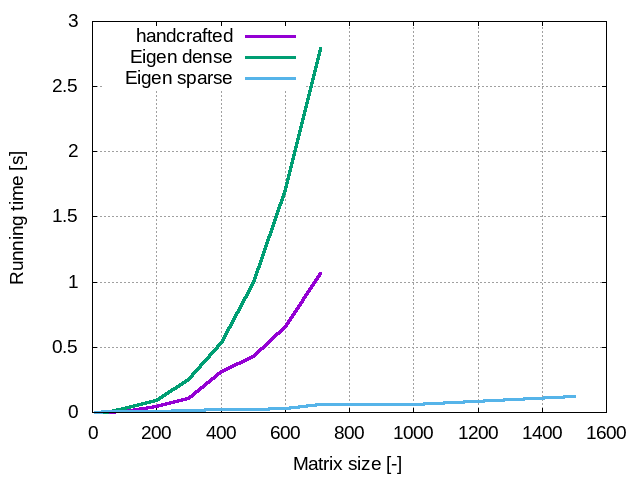
Wow! That is really impressive! To help you have a better feeling about how a better performance it is, look at the folowing graph. It compares the running times of the three examples we looked at. It shows that thinking a little bit to adopt the most appropriate srategy really pays off!
To conclude
I would say that, unless you have plenty of time, energy and experience and/or that you have very specific performance needs that are not covered by any linear algebra library such as Eigen: do not implement your own resolutions. Also, keep in mind that Eigen is not the only linear algebra library and that it has its own limitations but one can safely say that everything that have been written above is applicable to any similar library.
If you are interested, you can find all the code of this post on my github.
Have fun!
BONUS just for fun, check the folowing "matrixless" implementation of the random tridiagnal MxM matrix LU factorization and resolution.
#include <iostream>
#include <chrono>


void lu_factorization(int N, double * pa, double * pb, double * pc){
pc[0]=pc[0]/pb[0];
pb[0]=pb[0];
for(int i=1; i<=N; i++){
    pb[i]=pb[i]-pa[i]*pc[i-1];
    pc[i]=pc[i]/pb[i];
}
}

void forward(int N, double * pa, double * pb, double * pf){
pf[0]=pf[0]/pb[0];
for(int i=1; i<=N; i++){
    pf[i]=(pf[i]-pa[i]*pf[i-1])/pb[i];
}
}

void backward(int N, double * pc, double * pf){
for(int i=N-1; i>=0; i--){
    pf[i]=pf[i]-pc[i]*pf[i+1];
}
}

int main(){
int M=1500;
std::cout << "Matrix size M: " << M << std::endl;
srand(time(NULL));

auto tbegin = std::chrono::high_resolution_clock::now();
double * a = new double[M+1];
double * b = new double[M+1];
double * c = new double[M+1];
double * f = new double[M+1];

a[0]=0.0;
for(int i=1; i<=M; i++){
    a[i]=-1.;
}

b[M]=1.0;
for(int i=0; i<M; i++){
    b[i]=rand() % 9 + 1;
}

c[M]=0.0;
for(int i=0; i<M; i++){
    c[i]=-1.;
}

f[0]=1.0;
for(int i=1; i<=M; i++){
    f[i]=0.;
}

lu_factorization(M, a, b, c);
forward(M, a, b,f);
backward(M, c, f);

auto tend = std::chrono::high_resolution_clock::now();
std::chrono::duration<float> duration = tend-tbegin;
std::cout << "execution time (s): " << duration.count() << std::endl;
return 0;
}
You probably noted that its time and space complexity is O(n) so it is much MUCH faster than the previous handcrafted implementation, and even as Eigen Sparse's.
Matrix size M: 1500
execution time (s): 0.000184885
You can often write something faster than a linear algebra library when you focus on a very specific problem, indeed this works fine for a tridiagonal matrix, it can be adapted for a k-diagonal matrix (needs some work) but it is totally useless in the case of a matrix with randomly distributed non-zero terms whereas Eigen will still work.